CELLxGENE: scRNA-seq
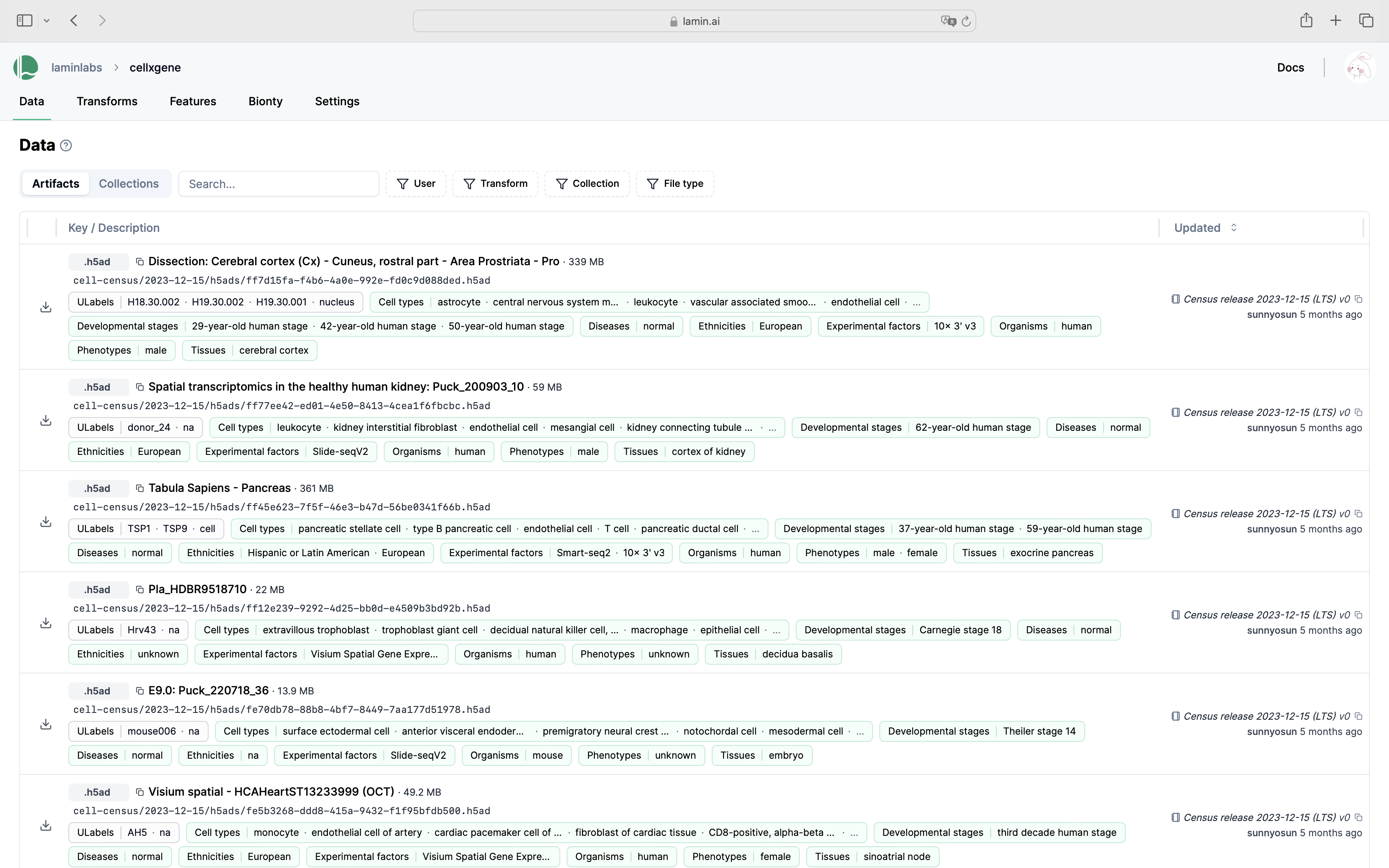
CZ CELLxGENE hosts the globally largest standardized collection of scRNA-seq datasets.
LaminDB makes it easy to query the CELLxGENE data and integrate it with in-house data of any kind (omics, phenotypes, pdfs, notebooks, ML models, …).
You can use the CELLxGENE data in two ways:
Query collections of
AnnDataobjects.Slice a big array store produced by concatenated
AnnDataobjects viatiledbsoma.
If you are interested in building similar data assets in-house:
See the transfer guide to zero-copy data to your own LaminDB instance.
See the scRNA guide to create a growing, standardized & versioned scRNA-seq dataset collection.
Show me a screenshot
Connect to the public LaminDB instance that mirrors cellxgene:
# pip install 'lamindb[bionty,jupyter]'
!lamin connect laminlabs/cellxgene
import lamindb as ln
import bionty as bt
Query & understand metadata
Auto-complete metadata
You can create look-up objects for any registry in LaminDB, including basic biological entities and things like users or storage locations.
Let’s use auto-complete to look up cell types:
Show me a screenshot
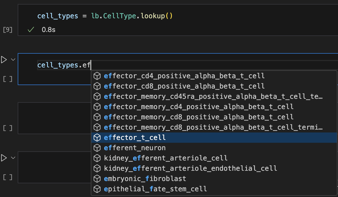
cell_types = bt.CellType.lookup()
cell_types.effector_t_cell
You can also arbitrarily chain filters and create lookups from them:
users = ln.User.lookup()
organisms = bt.Organism.lookup()
experimental_factors = bt.ExperimentalFactor.lookup()  # labels for experimental factors
tissues = bt.Tissue.lookup()  # tissue labels
suspension_types = ln.ULabel.filter(type__name="SuspensionType").lookup()
# here we choose to return .name directly
features = ln.Feature.lookup(return_field="name")
assays = bt.ExperimentalFactor.lookup(return_field="name")
Search & filter metadata
We can use search & filters for metadata:
bt.CellType.search("effector T cell").df().head()
And use a uid to filter exactly one metadata record:
effector_t_cell = bt.CellType.get("3nfZTVV4")
effector_t_cell
Understand ontologies
View the related ontology terms:
effector_t_cell.view_parents(distance=2, with_children=True)

Or access them programmatically:
effector_t_cell.children.df()
Query for individual datasets
Every individual dataset in CELLxGENE is an .h5ad file that is stored as an artifact in LaminDB. Here is an exemplary query:
ln.Artifact.filter(
    suffix=".h5ad",  # filename suffix
    description__contains="immune",
    size__gt=1e9,  # size > 1GB
    cell_types__in=[
        cell_types.b_cell,
        cell_types.t_cell,
    ],  # cell types measured in AnnData
    created_by=users.sunnyosun,  # creator
).order_by("created_at").df(
    include=["cell_types__name", "created_by__handle"]  # join with additional info
).head()
What happens under the hood?
As you saw from inspecting ln.Artifact, ln.Artifact.cell_types relates artifacts with bt.CellType.
The expression cell_types__name__in performs the join of the underlying registries and matches bt.CellType.name to ["B cell", "T cell"].
Similar for created_by, which relates artifacts with ln.User.
To see what you can query for, look at the registry representation.
ln.Artifact
Slice an individual dataset
Let’s look at an artifact and show its metadata using .describe().
artifact = ln.Artifact.get(description="Mature kidney dataset: immune", is_latest=True)
artifact.describe()
More ways of accessing metadata
Access just features:
artifact.features
Or get labels given a feature:
artifact.labels.get(features.tissue).df()
If you want to query a slice of the array data, you have two options:
Cache the artifact on disk and return the path to the cached data. Doesn’t download anything if the artifact is already in the cache.
Cache & load the entire artifact into memory via
artifact.load() -> AnnDataStream the array using a (cloud-backed) accessor
artifact.open() -> AnnDataAccessor
Both will run much faster in the AWS us-west-2 data center.
Cache:
cache_path = artifact.cache()
cache_path
Cache & load:
adata = artifact.load()
adata
Now we have an AnnData object, which stores observation annotations matching our artifact-level query in the .obs slot, and we can re-use almost the same query on the array-level.
See the array-level query
adata_slice = adata[
    adata.obs.cell_type.isin(
        [cell_types.dendritic_cell.name, cell_types.neutrophil.name]
    )
    & (adata.obs.tissue == tissues.kidney.name)
    & (adata.obs.suspension_type == suspension_types.cell.name)
    & (adata.obs.assay == experimental_factors.ln_10x_3_v2.name)
]
adata_slice
See the artifact-level query
collection = ln.Collection.filter(name="cellxgene-census", version="2024-07-01").one()
query = collection.artifacts.filter(
    organism=organisms.human,
    cell_types__in=[cell_types.dendritic_cell, cell_types.neutrophil],
    tissues=tissues.kidney,
    ulabels=suspension_types.cell,
    experimental_factors=experimental_factors.ln_10x_3_v2,
)
AnnData uses pandas to manage metadata and the syntax differs slightly. However, the same metadata records are used.
Stream, slice and load the slice into memory:
with artifact.open() as adata_backed:
    display(adata_backed)
We now have an AnnDataAccessor object, which behaves much like an AnnData, and slicing looks similar to the query above.
See the slicing operation
adata_backed_slice = adata_backed[
    adata_backed.obs.cell_type.isin(
        [cell_types.dendritic_cell.name, cell_types.neutrophil.name]
    )
    & (adata_backed.obs.tissue == tissues.kidney.name)
    & (adata_backed.obs.suspension_type == suspension_types.cell.name)
    & (adata_backed.obs.assay == experimental_factors.ln_10x_3_v2.name)
]

adata_backed_slice.to_memory()
Query collections of datasets
Let’s search collections from CELLxGENE within the 2024-07-01 release:
ln.Collection.filter(version="2024-07-01").search("human retina", limit=10)
Let’s get the record of the top hit collection:
collection = ln.Collection.get("quQDnLsMLkP3JRsC8gp4")
collection
It’s a Science paper and we can find more information on it using the DOI or CELLxGENE collection id. There are multiple versions of this collection.
collection.versions.df()
The collection groups artifacts.
collection.artifacts.df()
Let’s now look at the collection that corresponds to the cellxgene-census release of .h5ad artifacts.
collection = ln.Collection.get(key="cellxgene-census", version="2024-07-01")
collection
You can count all contained artifacts or get them as a dataframe.
collection.artifacts.count()
collection.artifacts.df().head() # not tracking run & transform because read-only instance
You can query across artifacts by arbitrary metadata combinations, for instance:
query = collection.artifacts.filter(
    organisms=organisms.human,
    cell_types__in=[cell_types.dendritic_cell, cell_types.neutrophil],
    tissues=tissues.kidney,
    ulabels=suspension_types.cell,
    experimental_factors=experimental_factors.ln_10x_3_v2,
)
query = query.order_by("size")  # order by size
query.df().head()  # convert to DataFrame
Slice a concatenated array
Let us now use the concatenated version of the Census collection: a tiledbsoma array that concatenates all AnnData arrays present in the collection we just explored. Slicing tiledbsoma works similar to slicing DataFrame or AnnData.
value_filter = (
    f'{features.tissue} == "{tissues.brain.name}" and {features.cell_type} in'
    f' ["{cell_types.microglial_cell.name}", "{cell_types.neuron.name}"] and'
    f' {features.suspension_type} == "{suspension_types.cell.name}" and {features.assay} =='
    f' "{assays.ln_10x_3_v3}"'
)
value_filter
'tissue == "brain" and cell_type in ["microglial cell", "neuron"] and suspension_type == "cell" and assay == "10x 3\' v3"'
Query for the tiledbsoma array store that contains all concatenated expression data. It’s a new dataset produced by concatenating all AnnData-like artifacts in the Census collection.
census_artifact = ln.Artifact.get(description="Census 2024-07-01")
Run the slicing operation.
human = "homo_sapiens"  # subset to human data

# open the array store for queries
with census_artifact.open() as store:
    # read SOMADataFrame as a slice
    cell_metadata = store["census_data"][human].obs.read(value_filter=value_filter)
    # concatenate results to pyarrow.Table
    cell_metadata = cell_metadata.concat()
    # convert to pandas.DataFrame
    cell_metadata = cell_metadata.to_pandas()

cell_metadata.head()
Create an AnnData object.
from tiledbsoma import AxisQuery

with census_artifact.open() as store:
    experiment = store["census_data"][human]
    adata = experiment.axis_query(
        "RNA", obs_query=AxisQuery(value_filter=value_filter)
    ).to_anndata(
        X_name="raw",
        column_names={
            "obs": [
                features.assay,
                features.cell_type,
                features.tissue,
                features.disease,
                features.suspension_type,
            ]
        },
    )

adata.var = adata.var.set_index("feature_id")
adata
! run input wasn't tracked, call `ln.track()` and re-run
AnnData object with n_obs × n_vars = 66418 × 60530
    obs: 'assay', 'cell_type', 'tissue', 'disease', 'suspension_type'
    var: 'soma_joinid', 'feature_name', 'feature_length', 'nnz', 'n_measured_obs'
Train ML models
You can either directly train ML models on very large collections of AnnData-like artifacts or on a single concatenated tiledbsoma-like artifact. For pros & cons of these approaches, see this blog post.
On a collection of arrays
mapped() caches AnnData objects on disk and creates a map-style dataset that performs a virtual join of the features of the underlying AnnData objects.
from torch.utils.data import DataLoader

census_collection = ln.Collection.get(name="cellxgene-census", version="2024-07-01")

dataset = census_collection.mapped(obs_keys=[features.cell_type], join="outer")

dataloader = DataLoader(dataset, batch_size=128, shuffle=True)

for batch in dataloader:
    pass

dataset.close()
For more background, see Train a machine learning model on a collection.
On a concatenated array
You can create streaming PyTorch dataloaders from tiledbsoma stores using cellxgene_census package.
import cellxgene_census.experimental.ml as census_ml

store = census_artifact.open()

experiment = store["census_data"][human]
experiment_datapipe = census_ml.ExperimentDataPipe(
    experiment,
    measurement_name="RNA",
    X_name="raw",
    obs_query=AxisQuery(value_filter=value_filter),
    obs_column_names=[features.cell_type],
    batch_size=128,
    shuffle=True,
    soma_chunk_size=10000,
)
experiment_dataloader = census_ml.experiment_dataloader(experiment_datapipe)

for batch in experiment_dataloader:
    pass

store.close()
For more background see this guide.